In our work on text-based geotagging, where many texts lack clear location references, having accurate uncertainty estimation is particularly valuable. In this blog post, we'll dive into different methods of achieving that.

To make it easy to follow along, we'll conduct all our experiments on a multi-class sentiment classification task.

Introduction

If you've ever worked with machine learning models, you know they're not just about making predictions; it's also crucial to understand how confident one can be in these predictions. This is where uncertainty estimation comes into play.

To illustrate the idea of uncertainty estimation, take a look at the bar charts below. We processed three different texts with the same model, and you can see that each text shows different confidence levels.

After reading this blog, you should have a clear understanding of different techniques, their strengths, weaknesses, and practical applications.

So, whether you're a seasoned data scientist or just dipping your toes into natural language processing (NLP), there's something here for everyone.

Setting up the environment

Let's start by setting up the environment.

Install the essential libraries for transformer-based text classification.

!pip install transformers datasets > /dev/null

Initialize the model and the tokenizer.

In this example, we're using a DistilBERT-based model, renowned for its efficiency in understanding and processing language.

import torch
from transformers import AutoTokenizer, AutoModelForSequenceClassification
from datasets import load_dataset
import random
import numpy as np

def initialize_model_and_tokenizer(device):
    tokenizer = AutoTokenizer.from_pretrained("bdotloh/distilbert-base-uncased-empathetic-dialogues-context")
    model = AutoModelForSequenceClassification.from_pretrained("bdotloh/distilbert-base-uncased-empathetic-dialogues-context").to(device)
    return model, tokenizer

device = 'cuda' if torch.cuda.is_available() else 'cpu'

# Use the functions to initialize the model and tokenizer, and prepare the dataset
model, tokenizer = initialize_model_and_tokenizer(device)

For this experiment, we're using a dataset from 'empathetic-dialogues-contexts'. It's a rich dataset with 32 distinct emotion labels, offering a diverse range of contexts and emotional nuances. To collect the dataset, respondents were asked to describe events associated with specific emotions. It consists of 19,209 texts for training, 2,756 texts for validation, and 2,542 texts for tests.
After initializing the environment, the model, and the dataset, let's set a seed value to ensure consistent results across runs.

def prepare_datasets():
    full_dataset = load_dataset("bdotloh/empathetic-dialogues-contexts", split='validation')
    shuffled_dataset = full_dataset.shuffle(seed=42)
    valid_dataset = shuffled_dataset.select(range(1000))
    train_dataset = load_dataset("bdotloh/empathetic-dialogues-contexts", split='train')
    return train_dataset, valid_dataset

# Define a seed for reproducibility
def set_seed(seed_value):
    random.seed(seed_value)
    np.random.seed(seed_value)
    torch.manual_seed(seed_value)
    if torch.cuda.is_available():
        torch.cuda.manual_seed_all(seed_value)

set_seed(0)  # Set the seed for reproducibility
train_dataset, valid_dataset = prepare_datasets()

Next, streamline the code by introducing several functions.

To view the complete code of the functions, refer to the notebook.

# Function to tokenize the dataset and return tensors ready for model input
def tokenize_data(tokenizer, dataset, max_length=512):
# Function to perform model predictions and return logits
def get_model_predictions(model, inputs, device):
# Function to calculate top-k accuracy
def calculate_top_k_accuracy(true_labels, predicted_probs, k=1):
# Function to calculate and print calibration metrics for different top percentages
def calculate_and_print_calibration_metrics(predictions, method_name, percentages=[5, 10, 25, 50]):
# Function to prepare the DataLoader for auxiliary model training
def create_data_loader(hidden_states, labels, batch_size=16):
# Function to calculate entropy from logits
def calculate_entropy(logits):
# Renders the calibration chart
def render_calibration_chart(predictions, method_name):

Uncertainty Estimation Methods

Now that the environment is ready, let's delve into the theory behind uncertainty estimation methods. We'll start with the simple techniques, discussing the intricacies and effectiveness of each.

Softmax-Based Methods

Softmax is a mathematical function that converts raw model logits into probabilities by exponentiating and normalizing them, ensuring a 0 to 1 range with a sum of 1. This makes it a crucial bridge between raw predictions and their interpretation as confidence levels across different classes.

Max Softmax

The Max Softmax method gauges uncertainty by relying on the highest softmax score to indicate confidence. This approach assumes that a higher probability for a class corresponds to greater certainty.

While computationally efficient and easy to implement, it may lack reliability, particularly for out-of-distribution samples where it tends to be overly confident.
In a graphical representation, imagine the Max Softmax method as assessing the length of the longest horizontal bar, with each bar length representing the model's confidence.

Softmax Difference

The Softmax Difference method extends the Max Softmax concept by assessing the difference between the highest and second-highest softmax probabilities. A significant gap between these probabilities signals a strong preference by the model for one class, implying heightened confidence.

This approach can offer a more nuanced measure of uncertainty compared to Max Softmax alone, particularly when the top two probabilities are closely matched.
To visualize this, picture the Softmax Difference method as examining the gap between two adjacent horizontal bars. A wider gap signifies a more decisive prediction from the model.

Softmax Variance

Softmax Variance considers the distribution of probabilities across all classes. It evaluates confidence spread by calculating the variance of softmax probabilities.

Low variance implies concentrated predictions, indicating high confidence in a specific class. High variance suggests uncertainty, with probabilities spread across multiple classes.

For a visual representation, imagine Softmax Variance as assessing the evenness of bar lengths across the chart. Greater uniformity signifies increased uncertainty in the model's predictions.

Softmax Entropy

Entropy measures the uncertainty in the model's predictions by considering the entire softmax probability distribution. High entropy corresponds to greater uncertainty.

Imagine Softmax Entropy as assessing the variation in the lengths of horizontal bars. A more scattered pattern indicates higher uncertainty.

Now that we've covered the conceptual basis of the uncertainty estimation methods, let's delve into the practical aspects.

def compute_confidence_scores(logits, method='max_softmax'):
    confidences = []
    if method == 'Max Softmax':
        confidences = torch.nn.Softmax(dim=-1)(logits).max(dim=1).values.cpu().numpy()
    elif method == 'Softmax Difference':
        top_two_probs = torch.topk(torch.nn.Softmax(dim=-1)(logits), 2, dim=1).values
        confidences = (top_two_probs[:, 0] - top_two_probs[:, 1]).cpu().numpy()
    elif method == 'Softmax Variance':
        probs = torch.nn.Softmax(dim=-1)(logits).cpu().numpy()
        confidences = np.var(probs, axis=1)
    elif method == 'Softmax Entropy':
        probs = torch.nn.Softmax(dim=-1)(logits)
        confidences = (probs * torch.log(probs)).sum(dim=1).cpu().numpy()
    else:
        raise ValueError(f"Unknown method {method}")
    return confidences

In many cases, various methods for uncertainty estimation share similar conclusions. However, it's the moments of disagreement that are particularly insightful.

In the example below, Max Softmax and Softmax Difference methods disagree on whether to include a text in Top-10% by confidence, allowing to explore the difference in the two assessments.

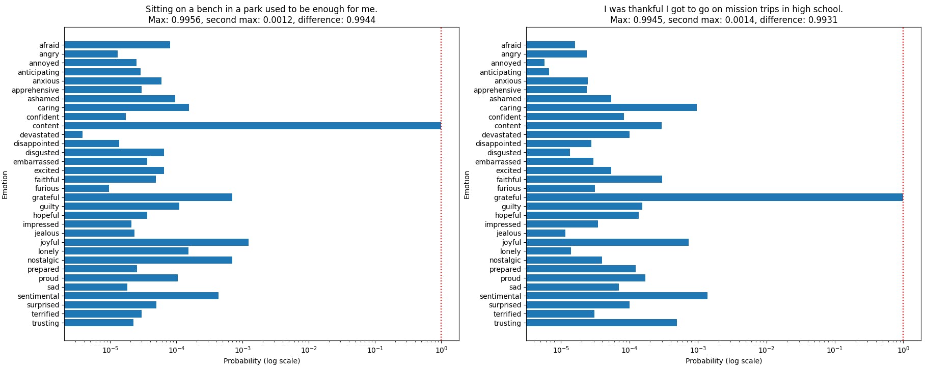
On the validation set, Top-10% threshold for Max-Softmax is 0.9941 and for Softmax Difference it is 0.9932.

On the left chart, both Max Softmax and Softmax Difference methods agree on identifying a sample text as one of the top 10% most confident predictions in the dataset, a consensus observed in 99% of the samples.
If the threshold value is set to the 10% most confident predictions, the "Content" class on the left chart surpasses for both the Max Softmax and Softmax Difference.
In contrast, the right chart shows the class "Grateful" surpassing the Max Softmax threshold with a value of 0.9945, but its difference of 0.9931 falls just short of the Softmax Difference threshold value.

Even though transformers often generate high probability values, a minor difference, such as the one between 0.9956 and 0.9945, can be crucial in the analysis. This highlights the importance of subtle probability variations when identifying the most confident predictions.

Advanced Methods

After exploring simple techniques that rely solely on a model's output from a single forward pass, let's step into a more advanced territory.

The next methods offer a deeper dive into uncertainty estimation.

Monte Carlo Dropout

Monte Carlo Dropout (MCD) estimates uncertainty by utilizing dropout layers in a neural network. It keeps dropout active during inference, running multiple forward passes to measure prediction variability. High variability signals low confidence.

MCD offers a practical method for quantifying model uncertainty without retraining or altering the model architecture.

During training, MCD uses dropout to regularize the model, preventing overfitting. Enabling dropout during inference simulates a model ensemble, where each pass uses a slightly different network architecture. The variance in predictions indicates the model's uncertainty.

Limitations and Assumptions:

Monte Carlo Dropout has a limitation in assuming that dropout layers alone can adequately capture model uncertainty. This assumption may not hold for all network architectures or datasets.
Another drawback is the increased computational cost due to the necessity for multiple forward passes.

# This pseudocode illustrates the core steps of Monte Carlo dropout 
def monte_carlo_dropout(model, data, num_samples):
    enable_dropout(model)
    for each sample in data:
        for j in 1 to num_samples:
            prediction_j = model_predict(sample)
            store prediction_j
        average_predictions = calculate_mean(predictions)
        uncertainty = calculate_standard_deviation(predictions)
        store average_predictions and uncertainty
    return aggregated_results

Mahalanobis Distance

The Mahalanobis Distance method gauges uncertainty by measuring how far a new data point is from the distribution of a class in the hidden space of a neural network. Smaller distances indicate higher confidence.

This method is good at spotting out-of-distribution examples because it shows how unusual a point is compared to what the model has learned. Points far from any class mean are likely outliers or from a new distribution.
Mahalanobis Distance can be used in combination with other techniques.
As such, to simplify and speed up calculations, Principal Component Analysis (PCA) can be used to reduce the dimensionality of the feature space. This method concentrates on the most crucial directions while minimizing noise, assuming that these directions capture the essential aspects for uncertainty estimation.

# This pseudocode illustrates Mahalanobis distance for estimating confidence
def prepare_mahalanobis(data, n_components=0.9):
    # Compute hidden states for the dataset
    hidden_states = compute_hidden_states(data)

    # Apply PCA to reduce dimensionality
    pca = PCA(n_components=n_components)
    pca.fit(hidden_states)
    hidden_states_pca = pca.transform(hidden_states)

    # Calculate mean vector and precision matrix
    mean_vector = np.mean(hidden_states_pca, axis=0)
    covariance_matrix = np.cov(hidden_states_pca, rowvar=False)
    precision_matrix = np.linalg.inv(covariance_matrix)

    return mean_vector, precision_matrix, pca

def compute_mahalanobis_distance(samples_pca, mean_vector, precision_matrix):
    distances = []
    for sample in samples_pca:
        distance = mahalanobis(sample, mean_vector, precision_matrix)
        distances.append(distance)
    return np.array(distances)

# Usage:
mean_vector, precision_matrix, pca = prepare_mahalanobis(train_data)
# Transform validation data using trained PCA
validation_pca = pca.transform(validation_data)
# Compute distances
distances = compute_mahalanobis_distance(validation_pca, mean_vector, precision_matrix)

Auxiliary Classifier

An auxiliary classifier is a secondary model trained to predict the certainty of the primary model's predictions. It takes the hidden states of the main model as input and learns to distinguish between correct and incorrect predictions.

This approach directly models uncertainty and can be tailored to the specific distribution of the data. By learning from the main model's hidden representations, the auxiliary classifier can provide a more nuanced understanding of the model's confidence in its predictions.

Limitations and Assumptions:

If the auxiliary classifier overfits to the primary model's mistakes, it may inherit its biases, leading to overconfident incorrect predictions or underconfident correct predictions.
It's essential to ensure that the auxiliary classifier is trained with a representative and balanced dataset to mitigate this risk.

# Pseudo code for Auxiliary classifier method
# Define a simple MLP for binary classification
class SimpleMLP(nn.Module):
    def __init__(self, input_dim):
        super().__init__()
        self.layer1 = nn.Linear(input_dim, 32)  # First linear layer
        self.layer2 = nn.Linear(32, 1)  # Second linear layer, outputting a single value

    def forward(self, x):
        x = torch.relu(self.layer1(x))  # Apply ReLU activation after first layer
        x = torch.sigmoid(self.layer2(x))  # Apply sigmoid activation after second layer for binary output
        return x

# Function to create binary labels based on prediction correctness
def create_binary_labels(predicted_classes, true_labels):
    correct_predictions = (predicted_classes == true_labels).astype(int)  # 1 for correct, 0 for incorrect
    return correct_predictions

# Train the auxiliary classifier with the balanced dataset
def train_auxiliary_classifier(features, labels, epochs=10):
    model = SimpleMLP(input_dim=features.shape[1]).to(device)
    optimizer = torch.optim.Adam(model.parameters(), lr=0.001)
    criterion = nn.BCELoss()  # Binary cross-entropy loss for binary classification

    for epoch in range(epochs):
        model.train()  # Set model to training mode
        total_loss = 0
        for inputs, targets in train_loader:  # Assuming features and labels are loaded as batches
            inputs, targets = inputs.to(device), targets.to(device)  # Move data to the appropriate device
            optimizer.zero_grad()  # Clear gradients before each update
            outputs = model(inputs)  # Forward pass to get output
            loss = criterion(outputs, targets)  # Calculate loss between model predictions and true labels
            loss.backward()  # Calculate gradients
            optimizer.step()  # Update model parameters
            total_loss += loss.item()  # Aggregate loss

    return model

# Use the trained auxiliary classifier to estimate uncertainty
def estimate_uncertainty(model, features):
    model.eval()  # Switch model to evaluation mode
    with torch.no_grad():
        predictions = model(features)
    uncertainty = 1 - predictions  # Assuming higher prediction score means lower uncertainty
    return uncertainty

Comparative Analysis

Let's compare these methods based on two key metrics:

Accuracy of the top-X% most confident predictions
Calibration charts

	top_5%_accuracy	top_10%_accuracy	top_25%_accuracy
Max Softmax	0.980	0.960	0.864
Softmax Difference	0.980	0.970	0.856
Softmax Variance	0.980	0.960	0.864
Softmax Entropy	0.980	0.960	0.856
Monte Carlo Dropout	0.860	0.870	0.800
Mahalanobis Distance	0.700	0.650	0.684
Auxiliary Classifier	0.840	0.760	0.720

Accuracy

The comparative analysis has brought to light the varying efficacy of different uncertainty estimation methods in augmenting the prediction confidence.

Compared to the baseline model with a general accuracy of approximately 54.60%, the softmax-based methods (Max Softmax, Softmax Difference, Softmax Variance, and Softmax Entropy) stand out with a higher accuracy. These methods have achieved nearly perfect accuracy (98%) in the top 5% most confident predictions.

This highlights their effectiveness in discerning the most reliable predictions from the model's output.

On the other hand, Monte Carlo Dropout, Mahalanobis Distance, and Auxiliary Classifier have underperformed in comparison to their softmax-based counterparts on this specific metric.

This discrepancy could be attributed to a potential lack of sufficient training data, which is often crucial for these methods to refine their estimates of uncertainty.

It's important to note that, despite this performance gap, current research acknowledges scenarios where more advanced methods may outperform softmax-based approaches. In more a complex task, the capability of Monte Carlo Dropout, Mahalanobis Distance, and Auxiliary Classifier could be more evident, making them invaluable tools in certain contexts.

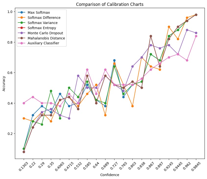
Calibration Charts

Calibration charts function like maps, helping to navigate the model's confidence reliability. They illustrate how closely the model's perceived confidence aligns with its actual accuracy. A well-calibrated model would have a chart where confidence levels match the accuracy.

Upon analyzing the calibration charts, each method shows strengths in calibration. The models confidence and actual accuracy align pretty well, which implies that all models are reasonably well-calibrated.

While there are expected fluctuations, they do not significantly diminish the overall calibration quality. It's reassuring that, regardless of the chosen method, a consistently reliable level of confidence in the model's predictions can be expected.

Conclusion

In this example task, different methods for uncertainty estimation have proven effective in boosting the reliability of predictions from transformer models. Even when a model has moderate overall performance, these methods can identify subsets of predictions with significantly higher accuracy.

Additional Reading and Practice Suggestions

For those who love a challenge and want to delve deeper, here are three research tasks:

Task 1. Bias Analysis

Investigate how the subset of most confident predictions differs from the full set. Which methods introduce more bias, and which are more impartial?

Task 2. Out-of-Distribution Performance

Test these methods on an out-of-distribution dataset. Choose a sentiment classification dataset, translate the current dataset, or craft a specific small dataset. How do the methods fare in unfamiliar waters?

Task 3. Kaggle Style Challenge

Blend the scores from different methods, add new features, and use them in a gradient boosting algorithm. Can you build a more accurate and robust ensemble compared to individual methods?

Yachay AI